Introduction to Intel pyDAAL
Raphael Cóbe, Silvio Stanzani, Jefferson Fialho, Rogério Iope
{rmcobe,silvio,jfialho,rogerio}@ncc.unesp.br
Source available on Github
Abstract
In this paper we intend to show how the python API of the Intel DAAL tool works. First, we explain how to manipulate data using the pyDAAL programming interface and then we show how to integrate it with python data manipulation/math APIs. Finally, we demonstrate how to use the Intel pyDAAL to implement a simple Linear Regression solution for a prediction problem.
1 Introduction
Data Science is a new recent field that put together lots of concepts of other areas such as: Data mining, Data Analysis, Data modeling, Data Prediction, Data Visualization and so on.
The need for performing such tasks as quickly as possible has become the main issue in today's data solutions. With that in mind, Intel has developed the Data Analytics Acceleration Library (DAAL), a highly optimized library whose goal is to provide a full solution for data analytics targeting today's highly parallel systems such as Intel Xeon Phi.
Intel DAAL delivers solutions for many steps of a data analytics pipeline, such as pre-processing, data transformations, dimensionality reduction, data modeling, prediction, and several drivers for reading and writing in most of the common data formats. A summary of all features inside the library can be seen in Figure 1.
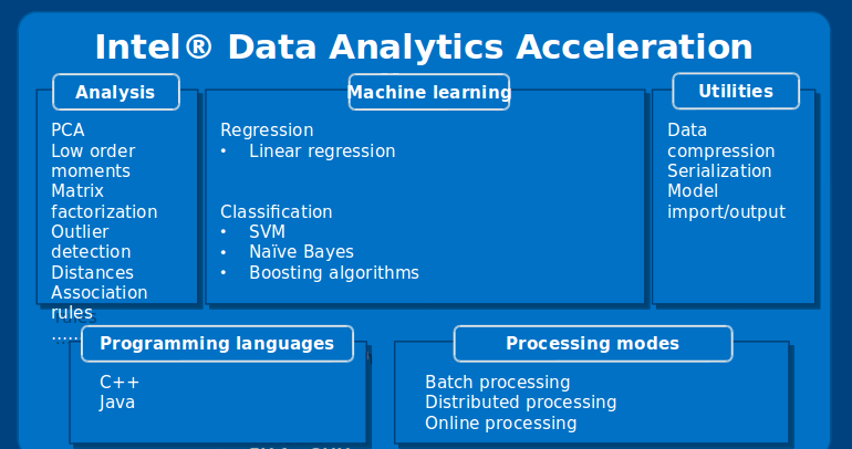
Figure 1. Main algorithms delivered by Intel DAAL
As can be seen in Figure 1, one can see that all APIs are compatible with C++, Java, and Python (a recent addition available from version 2017 beta). Many of the algorithms implemented inside the tool can be executed in 3 main modes:
- Batch: in this mode, the processing occurs in a serial way, e.g., the training algorithm is executed in a single node sequentially;
- Distributed: as the name suggests, in this processing mode, the dataset must be split and distributed among the computing nodes. The algorithm then calculate partial solutions and, at the last step, unifies such solutions; and
- Online: in this processing mode, the data is considered as being a continuous stream. The processing occurs by building incremental models, and, at the end, building a full model from the partial models.
More on the processing modes will be covered in this whitepaper.
The main goal of the Intel DAAL framework is to be able to cover most of the activities of a typical analytics pipeline such as the one seen on Figure 2.
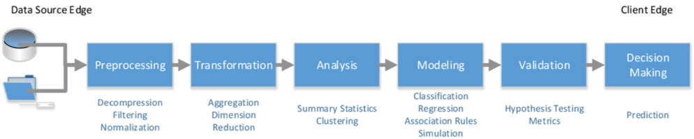
Figure 2. Typical Analytics Pipeline
The programming model imposed by this framework involves first reading the datasource and loading the correct data structures with the data. The datasource can either be in memory or in a persistent media such as a database or a CSV file. Then, we need to choose the algorithm for processing the data. In this step we need to specify the computation mode of our choice. Then we have to execute the chosen algorithm. After the execution is finished, depending on the computation mode specified, we may need to perform a merging step (computation finalization) in which, the partial results are used to produce a final result, e.g., building a final model of partial ones.
In the following sections we will explain each of the steps described above. It is not our intention to cover all of the algorithms available in the DAAL framework. For this paper we will show an example of linear regression on a batch computation mode.
1.1 The data used
In this paper we retrieved the data available at the UCI Machine Learning Repository that is used for prediction of residuary resistance of sailing yachts at the initial design stage. Such task is of a great value for evaluating the ship's performance and for estimating the required propulsive power.
Essentially, the inputs include the basic hull dimensions and the boat velocity.
The data set comprises of 308 full-scale observations. At each observation we have data for the following features:
- Longitudinal position of the center of buoyancy;
- Prismatic coefficient;
- Length-displacement ratio;
- Beam-draught ratio;
- Length-beam ratio; and
- Froude number.
- Residuary resistance per unit weight of displacement. (this is what we will try to predict)
The data used is available at: https://archive.ics.uci.edu/ml/datasets/Yacht+Hydrodynamics
2. Data Management
The main data abstraction used by the DAAL framework is called Numeric Table. It stores observations on lines and features on columns as can be seen in Figure 3. There are several specializations for this data structure optimized for specific use cases. We will cover this latter.
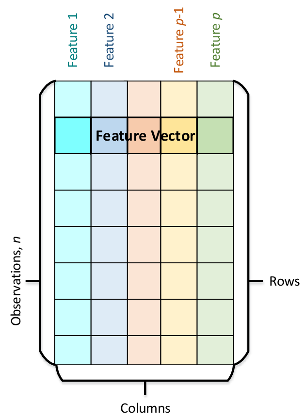
Figure 3. Numeric Table
Following a common usage of the framework, we first have to select the appropriate data source, which provides access for the data itself. It can be a data file, a database connection, a data stream, and so on. Intel DAAL data source interface provides support for 3 main data types: categorical, ordinal, and continuous. A data source main functionality is to stream data back and forward into memory.
The life cycle of a numeric table consists of the following major steps:
- Initialize: construct a numeric table (one has to provide the number of rows and columns);
- Operate: perform any operation needed on the data structure, such as data slicing; and
- Deinitialize: deallocate the memory used to store the data structure.
2.1 Main data structures
A numeric table is the key data structure on which the algorithms operate. Intel DAAL supports several specializations of a numeric data layout:
- Heterogeneous Tables: Structures of Arrays (SoA) and Arrays of Structures (AoS).
- Homogeneous Tables: dense and sparse.
- Matrices: dense matrix, packed symmetric matrix, and packed triangular matrices.
Essentially, Heterogeneous numeric tables allows one to store data features that are of different data types. Intel DAAL provides two ways to represent non-homogeneous numeric tables: Array of Structures - AOS and Structures of Arrays - SOA. AOS Numeric Table stores observations (feature vectors) in a contiguous memory block as can be seen in Figure 4.
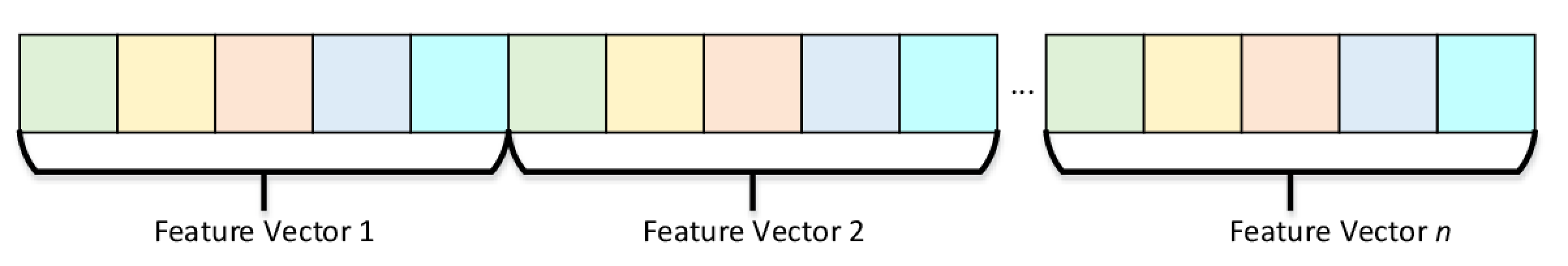
Figure 4. Array of Structures Numeric Table Representation
On the other hand, SOA Numeric Table stores data in a way that observations for each feature are laid out contiguously in memory, as can be seen in Figure 5.
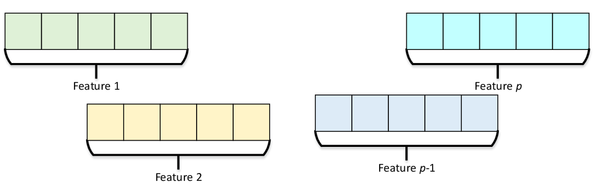
Figure 5. Structure of Arrays Numeric Table Representation
For the other basic data structures such as HomogenNumericTable class, and matrices such as PackedTriangularMatrix and PackedSymmetricMatrix, all the features are of the same basic data type. These data structures store values of the features in memory as one contiguous block in the row-major order.
In the context of the Intel DAAL, Matrix is a homogeneous numeric table most suitable for matrix algebra operations. A special treatment is given for special types of matrices such as triangular and symmetric. For those types, DAAL delivers implementations with reduced memory footprint using the special classes: PackedTriangularMatrix and PackedSymmetricMatrix.
2.2 Loading Data
In the following section we will present a few ways of reading data using the pyDAAL API. First we will show how to read data from a CSV file and how to perform simple data slicing operations on the data read. Then, we will show how to use data types from NumPy python API inside the DAAL framework.
2.2.1 From a CSV
CSV stands for comma separated values and as the name suggests, in this file, the feature values for each observation are separated by commas. Conversely, each observation is presented in one line, i.e, after the last feature value, the line is broken into a new one that will present the next observation features values. This file format is one of the most commonly used file formats.
In order to read from a CSV file, we first need to instantiate a new FileDataSource. We have to feed the data source with the name of the CSV file. We also have to define whether or not the dataset metadata (Dictionary) and the NumericTable are automatically created from the CSV.
from daal.data_management import FileDataSource
from daal.data_management import HomogenNumericTable
from daal.data_management import DataSourceIface
from daal.data_management import NumericTableIface

dataset_filename = 'yacht_hydrodynamics.csv'

yacht_datasource = FileDataSource(dataset_filename,
                            DataSourceIface.doAllocateNumericTable,
                            DataSourceIface.doDictionaryFromContext)

number_of_observations = yacht_datasource.loadDataBlock()

print("Observations read: {}".format(number_of_observations))
Listing 1. Reading from a CSV file
2.3 Integration with NumPy
NumPy is a widely spread API for manipulating multi-dimensional arrays. It is considered a common denominator in many numeric packages. Many tools for Machine Learning tasks use it directly or provide builtin methods for converting from or to NumPy arrays. Following we will show how to create NumericTables from the data inside a CSV file read using NumPy methods. Although, there is a limitation for creating NumericTables: the NumPy array has to be C-contiguous.
import numpy as np

data = np.genfromtxt('yacht_hydrodynamics.csv')
print("Is C Contiguous? {}".format(data.flags['C']))
data_nt = HomogenNumericTable(data)
print("Observations read: {}".format(data_nt.getNumberOfRows()))
Listing 2. Reading from a CSV file using NumPy
Listing 3 shows how to use a Pandas data frame for creating a NumericTable
import pandas as pd
from daal.data_management import HomogenNumericTable

dataframe = pd.read_csv('yacht_hydrodynamics.csv', delimiter=r"\s+")
numpy_array = dataframe.values
print("Is C Contiguous? {}".format(numpy_array.flags['C']))
numpy_array = np.ascontiguousarray(numpy_array, dtype = np.double) #Needs to convert to a C-Contiguous memory layout

array_nt = HomogenNumericTable(numpy_array)
print("Observations read: {}".format(array_nt.getNumberOfRows()))
Listing 3. Reading from a CSV file using Pandas dataframe
Another way to create a NumericTable is to provide the NumPy array directly to the constructor. Listing 4 shows how to do this. One very important remark that should be taken into account when building HomogenNumericTable from NumPy arrays is that it always requires the array to have the dimensions fully defined.
import numpy as np
from daal.data_management import HomogenNumericTable

numpy_array = np.array([1., 2., 3., 4., 5., 6.]).reshape(1, 6)
array_nt = HomogenNumericTable(numpy_array)
print("Dimensions: ({},{})".format(array_nt.getNumberOfRows(), array_nt.getNumberOfColumns()))
Listing 4. Generating a NumPy Array and creating a NumericTable from it.
It is also possible to extract a NumPy array from a NumericTable. The code in Listing 5 shows how to do that. First we need to use a BlockDescriptor and fill it with data from the NumericTable. It is important to stress that we have to specify the size of the block - the first parameter for the operation is the first row to load, and the second is the number of rows that will be loaded into the block. We can also specify the purpose of the block when we create it, e.g., in Listing 5 we specify that the block should not be used to update the table of the NumericTable. We do that by using the parameter readOnly - we could also have used the parameters readWrite or writeOnly.
In that sense, a BlockDescriptor works like a view of the dataset. It is important to note that after using the block, we need to release the allocated resources.
import numpy as np
from daal.data_management import BlockDescriptor_Float64, readOnly, HomogenNumericTable

block_descriptor = BlockDescriptor_Float64()
array_nt = HomogenNumericTable(np.array([1., 2., 3., 4., 5., 6.]).reshape(3,2))
array_nt.getBlockOfRows(0, array_nt.getNumberOfRows(), readOnly, block_descriptor)
numpy_array = block_descriptor.getArray()
array_nt.releaseBlockOfRows(block_descriptor)
print("Dimensions: {}".format(numpy_array.shape))
Listing 5. Building a NumPy array from a `NumericTable`
The pyDAAL API also allows one to integrate other types of NumericTables with specific data types such as sparse matrices from scipy.
In the following section we will present how to use pyDAAL to implement a linear regression on the example data used and described in Section 1.1.
3. Linear Regression
Inside any dataset into which we will try to make predictions, we have two types of variables: dependent and independent. The first one presents some dependency relationship (high correlation) with some or the combination of the others. The nature of this relationship is what we try to discover when we use a Machine Learning technique to make predictions based on the previous data.
For our example, we will employ a simple regression technique called Polynomial Linear Regression. In this method we use an algorithm that tries to fit a polynomial function to the data. That means that we will define the coeficients of an equation in the form $\theta_0 + \theta_1x_1 + \theta_2x_2 + ... + \theta_mx_m$ in order to approximate the behavior of our dependent variable inside our dataset, where $x_i$ is the i-th feature in our dataset.
In a more general definition, the problem which we are trying to solve is to estimate the value of $y$ (our dependent variable, or response), based on the observation $X$, also known as the feature vector.
For instance, we may want to use a regression technique to estimate the sales price of a land based on its location and its dimensions.
3.1 Linear Regression in Details
In order to use a regression based technique, we have to have a dataset for which we know the value of the dependent variable, e.g., we know the actual land prices for a few observations. Also, the value of the response should be continuous.
The problem we are addressing here is a minimization problem. Our goal is, at each step, to decrease the error in our equation for which the dependent variable is the result, e.g., assuming that we are fitting a linear model to our data. The error value of our model can be thought as the sum of all the errors for each data point. We can imagine this as the distance between our model equation line and the data points. That is the intuitive insight behind the fitting operation.
The error measure we have just described is called the squared error and is defined as:
Definition 1. Squared Error: Being the real value of the dependent variable defined as $y_i$ for $i \leq n$ where $n$ is the number of observations in our dataset. Being the value predicted by the model $\hat{y}_i$ for $i \leq n$, the Squared Error $\epsilon_i$ for the $i$-th observation is given as: $\epsilon_i = (y_i - \hat{y}_i)^2$. Thus, our global Squared Error is defined as: $E=\sum_{i=1}^{n}(y_i - \hat{y}_i)^2$.
In linear regression our challenge is to find the $\Theta$ vector which minimizes the error $E$ that we presented in Definition 1. In that case, the error $E$ can be seen as a function of $\theta_1, \theta_2, ..., \theta_m$. This is the function we are trying to minimize, i.e., $min(E(\Theta))$. This problem is called Multiple Linear Regression when we use several features to estimate the value of the dependent variable.
There are several algorithms for calculating the values of $\Theta$, one of the most popular is the Gradient Descent. Following we will give an intuition of how to solve the multiple linear regression problem using a technique called Normal Equation.
3.1.1 The Math Behind It
We first define that the value of our $i$-th response is defined as: $\hat{y}^{(i)} = \theta_0 x_0^{(i)} + \theta_1 x_1^{(i)} + \theta_2 x_2^{(i)}, ..., \theta_mx_m^{(i)}$. For notation, we will assume that $\Theta$ is the vector which contains the $\theta_m$ values. We will do the same with the features, defined inside the vector $X$, where each $x^{(i)}$ corresponds to the feature vector for the $i$-th observation. We will assume that $x_0^{(i)}=1$ for $i \leq n$, being $n$ the number of observations, i.e.:
$$ \Theta= \begin{bmatrix} \theta_0\\ \theta_1\\ \theta_2\\ ...\\ \theta_m\\ \end{bmatrix} ,\ X= \begin{bmatrix} x^{(1)}\\ x^{(2)}\\ x^{(3)}\\ ...\\ x^{(n)}\\ \end{bmatrix} ,\ Y= \begin{bmatrix} y^{(1)}\\ y^{(2)}\\ y^{(3)}\\ ...\\ y^{(n)}\\ \end{bmatrix} $$The $y^{(i)}$ dependent variable value is defined as $y^{(i)} = \hat{y}^{(i)} - \epsilon^{(i)}$.
Using a vector product notation we get: $Y = X\Theta - E$ and the Error function $E$ is defined as: $E(\Theta) = \sum_{i=1}^{m} (y^{(i)} - \Theta^T x^{(i)})^2$, or using the vector product notation we get that $E(\Theta) = (Y -X\Theta)^T(Y - X\Theta)$.
Since we are dealing with a minimization problem, we have to take partial derivatives $\frac{\partial}{\partial \theta_i}$ to solve for each $\theta_i$ value. Although the math behind this is quite simple we will not cover this demonstration in this paper. Please refer to http://eli.thegreenplace.net/2014/derivation-of-the-normal-equation-for-linear-regression for more details on how to solve this.
3.2 Linear Regression in Intel DAAL
After building a model, it is important that you are able to evaluate how good that model is. In order to do so, you should always split your dataset into a training partition, in which you will train your model, and a test partition, in which you will experiment the model and measure how good it is.
There is no rule of thumb when splitting the model. However, for most cases, a 20-80 split proportion is a good proportion. You should also be careful to draw random samples from your data in order to cover as much variance as possible. In Listing 6 we show how to draw samples from a data set using NumPy.
import numpy as np
import math
from numpy import genfromtxt
from daal.data_management import HomogenNumericTable

data = np.genfromtxt('yacht_hydrodynamics.csv')
sample = np.random.choice(len(data), size=math.floor(.8*len(data)), replace=False)

select = np.in1d(range(data.shape[0]), sample)

numpy_train_data = data[select,:]
numpy_test_data = data[~select,:]

train_data_table = HomogenNumericTable(data[select,:])
test_data_table = HomogenNumericTable(data[~select,:])

print("Number of Observations in Training Partition: {}".format(train_data_table.getNumberOfRows()))
print("Number of Observations in Test Partition: {}".format(test_data_table.getNumberOfRows()))
Listing 6. Drawing a random sample from a dataset using NumPy
In order to use pyDAAL algorithms we need to separate the dependent variable from the other features. Listing 7 shows how to cut a slice of the dataset. In this listing we use the same data read in Listing 6.
train_data_dependent_variable = numpy_train_data[:,6].reshape(246,1)

print("Dimension of the train_data dependent variable: {}".format(train_data_dependent_variable.shape))

train_data = np.delete(numpy_train_data, (6), axis=1)
print("Dimension of the train_data: {}".format(train_data.shape))


# We need to do the same with the test_data

test_data_dependent_variable = numpy_test_data[:,6].reshape(62,1)

print("Dimension of the test_data dependent variable: {}".format(test_data_dependent_variable.shape))

test_data = np.delete(numpy_test_data, (6), axis=1)
print("Dimension of the test_data: {}".format(test_data.shape))
Listing 7. Separating Variables
After separating the variables, we can create the instance of the algorithm in the previously chosen computation mode and train it as seen in Listing 8.
from daal.algorithms.linear_regression import training

train_data_table = HomogenNumericTable(train_data)
train_outcome_table = HomogenNumericTable(train_data_dependent_variable)

algorithm = training.Batch_Float64NormEqDense()

algorithm.input.set(training.data, train_data_table)

algorithm.input.set(training.dependentVariables, train_outcome_table)

trainingResult = algorithm.compute()

beta = trainingResult.get(training.model).getBeta()

block_descriptor = BlockDescriptor_Float64()

beta.getBlockOfRows(0, beta.getNumberOfRows(), readOnly, block_descriptor)

beta_coeficients = block_descriptor.getArray()

beta.releaseBlockOfRows(block_descriptor)

print("Coeficients: {}".format(beta_coeficients))
Listing 8. Training the Model
The values showed on Listing 8 are the $\theta_0, \theta_1, ..., \theta_m$ for the linear regression equation. Once we have such values it is time to test our model and try to predict the response in the test partition of our dataset. Listing 9 shows how to use the test partition to check our model quality.
from daal.algorithms.linear_regression import prediction

test_data_table = HomogenNumericTable(test_data)
test_outcome_table = HomogenNumericTable(test_data_dependent_variable)

algorithm = prediction.Batch()
algorithm.input.setTable(prediction.data, test_data_table)
algorithm.input.setModel(prediction.model,
                         trainingResult.get(training.model))

predictionResult = algorithm.compute()

test_result_data_table = predictionResult.get(prediction.prediction)

block_descriptor = BlockDescriptor_Float64()

test_result_data_table.getBlockOfRows(0, test_result_data_table.getNumberOfRows(),
                                      readOnly, block_descriptor)

numpy_test_result = block_descriptor.getArray()

test_result_data_table.releaseBlockOfRows(block_descriptor)

print("First 4 predicted values:")
print(numpy_test_result[1:4])
print("First 4 real responses:")
print(test_data_dependent_variable[1:4])
Listing 9. Predicting the Value of the Dependent Variable in the Test Partition
3.3 Evaluating the Model Quality
It is important to have ways of assessing the model quality. One of the mostly used metrics for doing so is the Root Mean Squared Error - RMSE. This measure uses the same unit as the dependent variable and basically shows the accumulated error value.
The RMSE, as its name suggests, is calculated as:
$$
RMSE = \sqrt{\frac{\sum_{i=1}^{n}(y^{(i)}-\hat{y}^{(i)})^2}{m}}
$$
We can define a function using the NumPy matrix operations capability as shown in Listing 10.
def RMSE(Y, Y_prime):
    return np.sqrt(np.mean((Y_prime - Y)**2))


print("RMSE: {}".format(RMSE(test_data_dependent_variable,numpy_test_result)))
Listing 10. RMSE function.
3.4 Improving the Model Quality with Polynomial Features Expansion
In some cases, the behavior of the data cannot be approximated using a linear function. A very popular technique for improving the model quality for those cases where linear functions are not enough is Polynomial Feature Expansion. In this technique we include derived features from the original dataset, changing the equation of the regression into a higher order polynomial. Thus, a polynomial expansion of second degree would introduce quadratic versions of the features.
The multiple linear regression equation shown - $y^{(i)} = \theta_0+\theta_1x_1^{(i)}+\theta_2x_2^{(i)}+...++\theta_mx_m^{(i)}$ becomes, in the quadratic expansion:
$$y^{(i)} = \theta_0+(\theta_1\ ^{(i)}x_1+\theta_2\ ^{(i)}x_1^2)+(\theta_3\ ^{(i)}x_2+\theta_4\ ^{(i)}x_2^2)+ ...+(\theta_{2m-1}\ ^{(i)}x_m+\theta_{2m}\ ^{(i)}x_m^2)$$Note that we used the superscript before the variable to denote the $i$-th observation. Luckly, most of the modern data manipulation APIs have a built-in function for performing such expansion. It is the case of the scikit-learn toolkit. In Listing 11 we show our previous examples using several degrees of polynomial expansions.
Unfortunately we were not able to do the expansion using the Normal Equation method. The pyDAAL reported that the it was not able to solve the linear system in order to calculate the $\Theta$ vector. Instead, we used the expansion with another type of Regression strategy, named Ridge regression. This type of regression is less susceptible to multicolinearity - a phenomenon that occurs when two or more features are extremely correlated. One can see that the Polynomial feature expansion, although improved a little the error, has no real effect on this type of regression.
We also were not able to expand even further the polynomial because the pyDAAL started to complain that the size of the NumericTable used for training the model was not correct. This must be due to a constraint on the number of features used.
from daal.algorithms.ridge_regression import training
from daal.algorithms.ridge_regression import prediction
from sklearn.preprocessing import PolynomialFeatures

train_outcome_table = HomogenNumericTable(train_data_dependent_variable)

for i in range(1,5):
    poly = PolynomialFeatures(degree=i)

    expanded_train_data = poly.fit_transform(train_data)
    train_data_table = HomogenNumericTable(expanded_train_data)

    algorithm = training.Batch()
    algorithm.input.set(training.data, train_data_table)
    algorithm.input.set(training.dependentVariables, train_outcome_table)

    training_model = algorithm.compute().get(training.model)

    expanded_test_data = poly.fit_transform(test_data)

    test_data_table = HomogenNumericTable(expanded_test_data)
    test_outcome_table = HomogenNumericTable(test_data_dependent_variable)

    prediction_algorithm = prediction.Batch()

    prediction_algorithm.input.setNumericTableInput(prediction.data, test_data_table)
    prediction_algorithm.input.setModelInput(prediction.model, training_model)

    prediction_result = prediction_algorithm.compute()

    test_result_data_table = prediction_result.get(prediction.prediction)
    block_descriptor = BlockDescriptor_Float64()
    test_result_data_table.getBlockOfRows(0, test_result_data_table.getNumberOfRows(),
                                              readOnly, block_descriptor)
    numpy_test_result = block_descriptor.getArray()
    test_result_data_table.releaseBlockOfRows(block_descriptor)

    print("{} degree of expanstion RMSE: {}".format(i, RMSE(test_data_dependent_variable,numpy_test_result)))
Listing 11. Polynomial Feature Expansion.
By using the scikit-learn API to perform the same operation, we were able to see that expanding the number of features by including their polynomial version could decrease the error. Such result can be seen in Listing 12. Also, it is easy to note that the optimal degree of expansion is 6. In the degrees of expansion 2, 3, and 4 the API also complained that it was not able to solve the linear system.
from sklearn.preprocessing import PolynomialFeatures
from sklearn import linear_model

for i in range(5,11):
    poly = PolynomialFeatures(degree=i)
    expanded_train_data = poly.fit_transform(train_data)

    regr = linear_model.LinearRegression()

    regr.fit(expanded_train_data, train_data_dependent_variable)

    numpy_test_result = regr.predict(poly.fit_transform(test_data))

    print("{} degree of expanstion RMSE: {}".format(i, RMSE(test_data_dependent_variable,numpy_test_result)))
Listing 12. Polynomial Feature Expansion using scikit-learn.
4. Conclusions
Intel has been developing a good framework for data science tasks. These tools are still on an early development stage, thus it easy to find some problems. This is specially true when using the pyDAAL that was officially released with Parallel Studio version 2017. The community is building around this tool once it provides a great level of integration with other Python tools.